Examples of Working in MathCAD
Most calculations in Mathcad can be performed in three ways:
– by selecting an operation from the menu, using
– toolbar buttons, or by accessing the corresponding functions.
Almost all operations assigned to menu items are duplicated by corresponding toolbar buttons. To access a built-in function, you can insert the function into the working document by selecting the desired name from the list of functions, enter the function name from the keyboard, or, for the most frequently used functions, insert the function name by clicking the button on the toolbar. Thus, in all three cases, the same workflow is followed:
a) an operation is selected by clicking the menu item or the button on the toolbar, after which, if necessary, the user has access to a drop-down menu or additional toolbar;
b) once an operation is selected, the user enters the required information in the dialog box or fills in the marked fields in the input field, which opens directly in the working document.
We will examine the contents of each menu item and describe the rules for performing the most frequently used operations.
Ranked Variables in MathCAD
MathCAD allows you to perform repeated calculations. This is done using a special type of variable—ranked variables, or discrete arguments.
A ranked variable accepts a range of values, for example, all integers from 0 to 10. If an expression contains a discrete argument (ranked variable), MathCAD evaluates the expression as many times as the discrete argument contains values.
Functions in MathCAD
The most common need in MathCAD is to use elementary functions. To use a function in an expression, you must specify the values of the input parameters in parentheses after the function name. The argument and value of elementary functions can be real or complex numbers. All angles are measured in radians.
Functions defined using the standard assignment sign are local, so they must be defined in the document before they are used.
Cartesian Coordinate Graphs in MathCAD
MathCAD allows you to plot two-dimensional graphs in Cartesian and polar coordinate systems, as well as three-dimensional graphs, including surface images, level maps, and many others. This operation is accessed through the Graph panel or through the corresponding Graphics menu item. In recent versions of the software, the Graph option is accessed through the Insert menu item.
Surface Graphs in MathCAD
Unlike two-dimensional graphs, which use discrete arguments and functions, a surface graph requires a matrix of values. Matrix elements are represented on the graph as heights located above or below the xy-plane. A typical surface plot shows the values of a function of two variables.
Solving Nonlinear Equations in MathCAD
Many equations, such as transcendental equations, do not have analytical solutions. However, they can be solved numerically using iterative methods with a specified error (the bisection method, the chord method, the tangent method, etc.). To solve a single equation f(x)=0 with one unknown, Mathcad uses the root function:
root(expression, variable_name)
The first argument is either a function defined elsewhere in the worksheet or an expression for calculating a scalar value. The second argument is the name of a variable used in the expression.
This variable must be assigned a numeric value before calling the root function. Mathcad uses this value as an initial guess when searching for the root. The root function returns the value of the variable that makes the expression evaluate to 0. Mathcad can find both real and complex roots. To find real roots, the initial guess must be real, and to find complex roots, it must be complex.
The precision of calculations is set by the TOL system variable, which can be changed by selecting Math – Options – Built-in Variables.
If Mathcad cannot find the root, an error message is displayed. This error may be caused by:
– the equation has no roots;
– the roots of the equation are located far from the initial guess;
– the expression has local extrema between the initial guess and the roots;
– the expression has discontinuities between the initial guess and the roots;
– the expression has a complex root, but the initial guess was real (or vice versa).
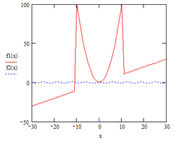
To avoid errors, it is recommended to first examine the graph of the function f(x). This allows you to determine the presence of roots of the equation f(x)=0 and, if present, determine their approximate values.
If you need to find multiple roots of the equation, you need to run the root function multiple times. Two approaches can be used:
1. Plot the graph of f(x), determine the root intervals, and run the root function multiple times with different initial guesses (you can choose one of the endpoints of the root interval as the initial guess).
2. Find one of the roots of the equation, specifying an arbitrary initial guess. For an equation f(x) with a known root a, finding additional roots is equivalent to finding the roots of the equation h(x)=0, where h(x)=f(x)/(x-a). This technique is convenient for finding roots of an equation that are located close to each other.
Solving Transcendental Equations in MathCAD
1. Separate the roots of the equation graphically over a given interval: reduce the equation to the form f(x)=0 and define the function of the left-hand side of the equation. Plot the graph of the function over the specified interval. From the graph, determine the initial approximation of the root(s), entering them into the variables x1 (x2, …).
2. For each initial approximation of the root, find a solution to the equation using the root function.
Solving Systems of Nonlinear Equations in MathCAD
Mathcad allows you to solve systems of equations. The maximum number of equations and variables is 200. This is accomplished using a special calculation block, in which, after the function word Given, the equations of the system and various constraints in the form of inequalities are specified. The block ends with a call to the Find function to find the solution:
Given
Equations and Inequalities
Expression with Find(x,y)
The Find function’s parameters are variables that are selected during the solution process to satisfy the system’s equations and inequalities. All variables before Given must be assigned initial values beforehand. When specifying equations, a special bold equal sign is used, which is entered with the keyboard shortcut Ctrl=. Constraint conditions are specified using relational operators selected in the Boolean panel.